Cohen’s $d$ in simple linear regression models

Cohen’s $d$ is a common measure of effect size. This short post illustrates the basic idea behind it and shows how to calculate it in R for effects estimated with simple linear regression models.

Consider a scenario with two conditions, control and treatment and some continuous outcome (e.g., weight). Cohen’s $d$ is then defined as:

$$d=\frac{\overline{x_1}-\overline{x_2}}{s}$$

where $\overline{x_1}$ and $\overline{x_2}$ are the means of the conditions and

$$s=\sqrt{\frac{(n_1-1)s_1^2+(n_2-1)s_2^2}{n_1+n_2-2}}$$

with $s_1$ and $s_2$ being the standard deviations and $n_1$ and $n_2$ the numbers of data points of the two conditions. The quantity $s$ is called the pooled standard deviation.

The definition above may not look terribly transparent, but conceptually $d$ is simply the size of the effect (i.e. the difference between control and treatment, $\overline{x_1}-\overline{x_2}$) relative to the variance that is left in the data after accounting for that effect. So the effect is basically taken from some absolute scale (e.g., kilograms) and is put on a scale that is relative to the variability in the particular data set.

Here’s an example to illustrate this. We use data from Annette Dobson (1990), An Introduction to Generalized Linear Models (p. 9, plant weight data).

ctl    <- c(4.17,5.58,5.18,6.11,4.50,4.61,5.17,4.53,5.33,5.14)
trt    <- c(4.81,4.17,4.41,3.59,5.87,3.83,6.03,4.89,4.32,4.69)
group  <- gl(2, 10, 20, labels=c("Ctl", "Trt"))
weight <- c(ctl, trt)
n      <- length(weight)

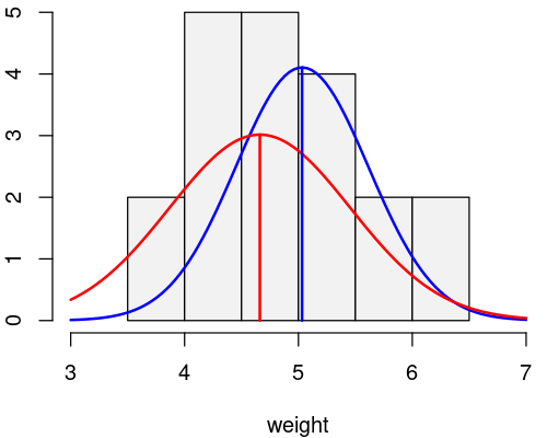
The by-conditions means and the plot below show that the average weight was somewhat lower in the treatment condition than in the control condition.

tapply(weight, group, mean)

  Ctl   Trt 
5.032 4.661

The standard deviation in the treatment condition (red) was also higher than in the control condition (blue).

Next, we fit a simple linear model to estimate this effect.

lm(weight ~ group) -> m
summary(m)

Call:
lm(formula = weight ~ group)

Residuals:
    Min      1Q  Median      3Q     Max 
-1.0710 -0.4938  0.0685  0.2462  1.3690 

Coefficients:
            Estimate Std. Error t value Pr(>|t|)    
(Intercept)   5.0320     0.2202  22.850 9.55e-15 ***
groupTrt     -0.3710     0.3114  -1.191    0.249    
---
Signif. codes:  0 ‘***’ 0.001 ‘**’ 0.01 ‘*’ 0.05 ‘.’ 0.1 ‘ ’ 1

Residual standard error: 0.6964 on 18 degrees of freedom
Multiple R-squared:  0.07308,	Adjusted R-squared:  0.02158 
F-statistic: 1.419 on 1 and 18 DF,  p-value: 0.249

With the default treatment coding, the intercept of this model ($5.03$) represents the mean weight in the control condition and the coefficient groupTrt ($-0.37$) how much smaller the weight was in the treatment condition. Note that the effect of the treatment is non-zero but at the same time non-significant.

Is this effect small or large? Let’s calculate Cohen’s $d$ to find out!

The approach below is going to look a bit different from the conventional definition of Cohen’s $d$ given above, but the result is the same and I think the approach below is more instructive. The idea is the following: We remove the effect of the treatment from the data and then we calculate the pooled standard deviation of the remaining data. Cohen’s $d$ is then simply $\frac{{\beta }_2}{s}$ where ${\beta }_2$ is the coefficient of the model that represents the effect of the treatment (groupTrt, the second coefficient of the model fit above).¹

coef(m)[2]          -> b  # Coefficient of interest
model.matrix(m)[,2] -> x  # Corresponding column of the design matrix
weight - b * x      -> y  # The data minus the effect of interest

The variable y now contains the data but without the effect of the treatment. Next, we calculate the pooled standard deviation. The recipe is the same as for the ordinary standard deviation, except that we divide by $n-2$ instead of $n-1$ (this is done to prevent bias):

$$s=\sqrt{\frac{1}{n-2}\sum _i^n{(y_i-\bar{y})}^2},$$

We’ll do this in two steps: First, we calculate the sum of squared errors (the right part under the square root), and then the pooled standard deviation:

sum((y - mean(y))^2) -> sse
sqrt(sse / (n-2))    -> sd.pooled
sd.pooled

[1] 0.6963895

Now, Cohen’s $d$ is simply:

b / sd.pooled -> d
d

groupTrt 
-0.5327478

The result, $-0.53$, is negative because the effect is negative-going. The magnitude (around ±0.5) is conventionally interpreted as a medium effect size. Note, however, that while the effect is of medium size, it’s at the same time not significant. It may be confusing to talk about the size of the effect when it’s not even clear whether the effect exists at all, but that’s simply a consequence of the fact that the word “effect” is doing double duty here. We use it to describe the observed difference in the sample, but in the context of inferential statistics, we use it for the hypothetical effect in the larger population, which may not exist.

While the procedure above produces the correct result, there is an alternative way to calculate Cohen’s $d$ that is perhaps conceptually even more transparent. The difference is in how the pooled standard deviation is calculated. This time we’re using the residuals of the linear model to calculate the squared errors.

sum(residuals(m)^2) -> sse
sqrt(sse / (n-2))   -> sd.pooled
sd.pooled

[1] 0.6963895

The result is exactly the same as before. What this illustrates is that, in this particular scenario (single regression), Cohen’s $d$ is really just the magnitude of the effect (in terms of the outcome scale) divided by the residual standard deviation, with the small difference that the standard deviation is the pooled variety, i.e. using division by $n-2$ instead of $n-1$, which makes the estimate unbiased.

Note, however, that the approach using residuals won’t work in a multiple regression setting where the residual variance is going to be smaller due to the other predictors present in the model. Nevertheless, I hope that this way of thinking about Cohen’s $d$ helps to understand and memorize the basic idea.

Finally, a word of caution: The code above is intended just for illustration purposes. For serious uses, I recommend existing R packages such as the effsize package. There are also different ways to calculate Cohen’s $d$ and for mixed models (a.k.a. hierarchical / multi-level models) there is no single agreed-upon method for calculating Cohen’s $d$ (see here for an interesting blog post about this issue). So the example above really just shows the simplest case.