Bayesian mixed-effects models using MCMCglmm (obsolete)
Note: I wrote this tutorial years ago ago when MCMCglmm was perhaps the best option for fitting Bayesian LMMs in R. In the meantime, much better alternatives have been developed, such brms, rstanarm, and rethinking. For this reason, I consider this tutorial obsolete.
The lme4 package for fitting (generalized) linear mixed-effects models has proven to be a powerful tool for analyzing data from experimental studies. However, most people encounter situations in which lme4 does not provide answers because the model-fitting process fails to converge. This is can be the case when the model is too complex to be supported by the available data. Bayesian implementations of mixed-effects models can help in some of these situations because mild priors on the random effects parameters can be used to constrain the search space. In non-technical terms, the Bayesian framework allows us to nudge the model fitting process in the right direction.
MCMCglmm is a package for fitting Bayesian mixed models in R and was written by Jarrod Hadfield. Its use is roughly similar to lme4’s but there are some additional complexities that the user has to deal with. This tutorial aims to get you started with MCMCglmm and shows how the Bayesian analogue of an lme4 model can be implemented with MCMCglmm.
However, there are more reasons for considering MCMCglmm than just converge issues in lme4. For example, MCMCglmm supports multi-variate dependent variables and a wide variety of distributions, for instance, multinominal, exponential, zero-inflated, and censored distributions. Further, MCMCglmm can be used to implement Hurdle models and models with heterogenous residual variances. In this tutorial, however, we will not make use of these capabilities but simply translate an lme4 model to MCMCglmm.
Note that this text is not supposed to be a self-contained introduction to Bayesian mixed models or MCMC sampling more generally. At some points we assume that the reader is at least vaguely familiar with the basic ideas behind these concepts. If you are not, give it a shot anyway, and google concepts that you are not familiar with. You can also consult the documentation of MCMCglmm:
Also feel free to use GitHub’s issue tracker to ask questions or to point out mistakes. If you want to submit a pull request with improvements, that would be great, too.
Finally, note that the complete code used in this tutorial is also available in a separate R file (README.R). You can download this file and execute the code in your favorite editor for R. The data can be found here.
Overview
To illustrate the use of MCMCglmm, we will analyze a data set from a language production experiment. In this experiment, the participants had to describe visual scenes. The aim was to determine the factors governing the participant’s use of pronouns (he, she, it, …) in their descriptions.
We first attempt an analysis using lme4 and we will see how and why this fails. Then we implement an analogous model using MCMCglmm. MCMCglmm does not perform automatic convergence checks like lme4 does, which means that it is our job to determine whether model fitting was successful. Since there are no definitive criteria for deciding whether the model has successfully converged, we have to make use of some heuristics. (Lme4 also uses heuristics for this purpose but this happens behind the scenes.) We first use some subjective heuristics and then a somewhat more principled criterion for determining convergence (Gelman-Rubin criterion). Finally, we evaluate the model with respect to the research question.
Design of the study and data
The experiment had a 2×2×2 design and the factors were a, b, and c. (The description of the experiment is censored because the study is not yet published. We might add more details once that has happened.) The factors a and b were within-item and c was between-items. All three factors are coded using -1 and 1. There were 71 subjects and 36 items, and each subject saw one version of each item. The dependent variable indicates for each trial whether or not the participant used a pronoun in his description of a visual scene (1 if a pronoun was used, 0 otherwise).
We first load the data and whip it into shape:
d <- read.table("data/data.tsv", sep="\t", head=T)
d$pronoun <- as.logical(d$pronoun)
head(d)
| subject | item | a | b | c | pronoun |
|---|---|---|---|---|---|
| 1 | 1 | -1 | 1 | -1 | FALSE |
| 1 | 3 | 1 | -1 | -1 | TRUE |
| 1 | 5 | -1 | 1 | -1 | TRUE |
| 1 | 7 | 1 | -1 | -1 | TRUE |
| 1 | 9 | -1 | 1 | -1 | FALSE |
| 1 | 11 | -1 | -1 | -1 | FALSE |
summary(d)
   subject           item             a                 b                  c            pronoun
Min.   : 1.00   Min.   : 1.00   Min.   :-1.0000   Min.   :-1.00000   Min.   :-1.0000   Mode :logical
1st Qu.:19.00   1st Qu.: 9.00   1st Qu.:-1.0000   1st Qu.:-1.00000   1st Qu.:-1.0000   FALSE:477
Median :36.00   Median :18.00   Median : 1.0000   Median :-1.00000   Median :-1.0000   TRUE :635
Mean   :35.89   Mean   :18.35   Mean   : 0.1421   Mean   :-0.02338   Mean   :-0.1241   NA's :0
3rd Qu.:54.00   3rd Qu.:27.25   3rd Qu.: 1.0000   3rd Qu.: 1.00000   3rd Qu.: 1.0000
Max.   :71.00   Max.   :36.00   Max.   : 1.0000   Max.   : 1.00000   Max.   : 1.0000
Proportions of pronoun responses per cell of the design:
x <- with(d, tapply(pronoun, list(a, b, c), mean))
dimnames(x) <- list(c("not-a", "a"), c("not-b", "b"), c("not-c", "c"))
x
| not.b.not.c | b.not.c | not.b.c | b.c | |
|---|---|---|---|---|
| not-a | 0.264705882352941 | 0.235294117647059 | 0.42 | 0.2 |
| a | 0.723404255319149 | 0.957746478873239 | 0.875816993464052 | 0.782945736434108 |
Looking at the contingency table below, we see that some cells of the design had very few measurements. In fact, only nine subjects contributed measurements to all cells of the design and nine contributed only to 4 of the 8 cells (second table below). The reason for these strong unbalances is that the factors a and b were not experimentally controlled but features of the utterances that the participants produced.
with(d, table(a, b, c))
| a | b | c | Freq | |
|---|---|---|---|---|
| 1 | -1 | -1 | -1 | 34 |
| 2 | 1 | -1 | -1 | 282 |
| 3 | -1 | 1 | -1 | 238 |
| 4 | 1 | 1 | -1 | 71 |
| 5 | -1 | -1 | 1 | 100 |
| 6 | 1 | -1 | 1 | 153 |
| 7 | -1 | 1 | 1 | 105 |
| 8 | 1 | 1 | 1 | 129 |
library(dplyr)

x <- d %>%
    group_by(subject) %>%
    summarize(nc = length(unique(paste(a,b,c))))

table(x$nc)
| Var1 | Freq |
|---|---|
| 4 | 9 |
| 5 | 9 |
| 6 | 26 |
| 7 | 18 |
| 8 | 9 |
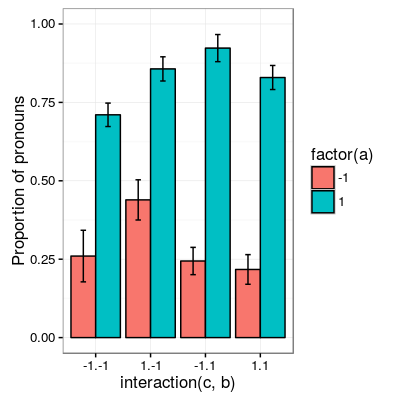
The following plot shows the proportion of pronoun responses in all cells of the design.
subject.means <- d %>%
    group_by(subject, c, a, b) %>%
    summarize(prop = mean(pronoun))

condition.means <- subject.means %>%
    group_by(c, a, b) %>%
    summarize(mean = mean(prop),
              se   = sd(prop)/sqrt(n()))

library(ggplot2)

ggplot(condition.means, aes(x=interaction(c, b), fill=factor(a), y=mean)) +
  geom_bar(stat="identity", pos="dodge", colour="black") +
  geom_errorbar(aes(ymin=mean-se, ymax=mean+se), size=.5, width=.2, position=position_dodge(.9)) +
  ylim(c(0,1)) +
  theme_bw(base_size=12) +
  ylab("Proportion of pronouns")
Attempt to model the data with lme4
In principle, lme4 can deal with unbalanced data sets but the low number of data points in some cells of the design means that it is hard to estimate some of the effects. One of these effects is the three-way interaction which depends on the proportions of pronouns in all cells of the design. Unfortunately, this three-way interaction was precisely the effect of interest in the study.
We start with the maximal model justified by the design:
library(lme4)
m1 <- glmer(pronoun ~  (a + b + c)^3            +
                      ((a + b + c)^3 | subject) +
                      ((a + b    )^2 | item),
            data=d, family="binomial")
A side note on the formula notation used above: (a + b + c)^3 is a little known alternative notation for a * b * c. So it gives us parameters for the main effects, the two-way interactions, and the three-way interaction. The benefit of this notation is that it is more convenient during the design stage of the model when we often change the structure of the model. For example if we want to exclude the three-way interaction, we can simply replace the 3 by a 2 ((a + b + c)^2) because what the exponent says is up to which level we want to include interactions.
The model above is the most complex model that can be fit given the design. The model has fixed effects terms for all three factors and all their interactions. Following Barr, Levy, Scheepers, Tily (2013), there are also random slopes for all these factors. The exception is c which was manipulated between items, so there can’t be by-item random-slopes for that factor or any interaction in which this factor is involved.
The attempt to fit this model takes about 30 minutes on my machine and ultimately fails with one of the most colorful collections of warning messages I have ever seen from lme4:
Warning messages:
1: In commonArgs(par, fn, control, environment()) :
  maxfun < 10 * length(par)^2 is not recommended.
2: In optwrap(optimizer, devfun, start, rho$lower, control = control,  :
  convergence code 1 from bobyqa: bobyqa -- maximum number of function evaluations exceeded
3: In (function (fn, par, lower = rep.int(-Inf, n), upper = rep.int(Inf,  :
  failure to converge in 10000 evaluations
Warning messages:
1: In checkConv(attr(opt, "derivs"), opt$par, ctrl = control$checkConv,  :
  unable to evaluate scaled gradient
2: In checkConv(attr(opt, "derivs"), opt$par, ctrl = control$checkConv,  :
  Model failed to converge: degenerate  Hessian with 4 negative eigenvalues
Ben Bolker, the current maintainer of the lme4 package, somewhere pointed out that the occurrence of a warning does not strictly imply that the model is degenerate, however, one of the above messages explicitly says that convergence failed and examining the model gives us good reasons to belief that:
summary(m1)
Generalized linear mixed model fit by maximum likelihood (Laplace Approximation) ['glmerMod']
 Family: binomial  ( logit )
Formula: pronoun ~ (a + b + c)^3 + ((a + b + c)^3 | subject) + ((a + b)^2 |      item)
   Data: d

     AIC      BIC   logLik deviance df.resid
  1015.3   1286.0   -453.6    907.3     1058

Scaled residuals:
    Min      1Q  Median      3Q     Max
-2.8041 -0.2491  0.0653  0.3344  3.3503

Random effects:
 Groups  Name        Variance Std.Dev. Corr
 subject (Intercept) 18.90141 4.3476
         a            5.92954 2.4351    0.75
         b            3.78364 1.9452    0.93  0.93
         c            7.29737 2.7014   -0.95 -0.89 -0.99
         a:b          7.02041 2.6496    0.94  0.86  0.96 -0.97
         a:c          4.46273 2.1125   -0.91 -0.93 -0.99  0.99 -0.99
         b:c          6.65586 2.5799   -0.90 -0.93 -0.99  0.99 -0.95  0.98
         a:b:c        8.12665 2.8507   -0.90 -0.93 -0.99  0.99 -0.96  0.99  1.00
 item    (Intercept)  0.07434 0.2726
         a            0.11726 0.3424   -1.00
         b            0.01363 0.1168   -1.00  1.00
         a:b          0.02852 0.1689   -1.00  1.00  0.99
Number of obs: 1112, groups:  subject, 71; item, 36

Fixed effects:
            Estimate Std. Error z value Pr(>|z|)
(Intercept)   2.7264     1.0488   2.599  0.00934 **
a             4.2605     0.9660   4.410 1.03e-05 ***
b             1.9254     0.9223   2.088  0.03684 *
c            -1.9351     0.9454  -2.047  0.04068 *
a:b           2.6403     0.9417   2.804  0.00505 **
a:c          -2.2455     0.9285  -2.418  0.01559 *
b:c          -2.6537     0.9632  -2.755  0.00587 **
a:b:c        -2.5660     0.9717  -2.641  0.00827 **
---
Signif. codes:  0 ‘***’ 0.001 ‘**’ 0.01 ‘*’ 0.05 ‘.’ 0.1 ‘ ’ 1

Correlation of Fixed Effects:
      (Intr) a      b      c      a:b    a:c    b:c
a      0.899
b      0.920  0.977
c     -0.959 -0.948 -0.962
a:b    0.959  0.948  0.956 -0.985
a:c   -0.923 -0.972 -0.986  0.957 -0.962
b:c   -0.937 -0.979 -0.980  0.964 -0.959  0.984
a:b:c -0.958 -0.957 -0.958  0.983 -0.978  0.962  0.967
convergence code: 0
unable to evaluate scaled gradient
Model failed to converge: degenerate  Hessian with 2 negative eigenvalues
failure to converge in 10000 evaluations

Warning messages:
1: In vcov.merMod(object, use.hessian = use.hessian) :
  variance-covariance matrix computed from finite-difference Hessian is
not positive definite or contains NA values: falling back to var-cov estimated from RX
2: In vcov.merMod(object, correlation = correlation, sigm = sig) :
  variance-covariance matrix computed from finite-difference Hessian is
not positive definite or contains NA values: falling back to var-cov estimated from RX
Almost all estimates of the correlations of random effects are close to -1 or 1 and all fixed effects are significant. Both is fairly implausible. The standard thing to do in this situation is to simplify the model until it converges without warnings. However, according to Barr et al., the only hard constraint is that the random slopes for the effect of interest (the effect about which we want to make inferences) need to be in the model. This is often overlooked because the title of the paper – Random effects structure for confirmatory hypothesis testing: Keep it maximal – leads many people to think that Barr et al. mandate maximal random effect structures no matter what.
In our case, the effect of interest is the three-way interaction and the simplest possible model is therefore the following:
m2 <- glmer(pronoun ~ (a + b + c)^3 +
                      (0 + a : b : c|subject) +
                      (0 + a : b : c|item),
            data=d, family="binomial")
Warning messages:
1: In commonArgs(par, fn, control, environment()) :
  maxfun < 10 * length(par)^2 is not recommended.
2: In (function (fn, par, lower = rep.int(-Inf, n), upper = rep.int(Inf,  :
  failure to converge in 10000 evaluations
Warning messages:
1: In checkConv(attr(opt, "derivs"), opt$par, ctrl = control$checkConv,  :
  unable to evaluate scaled gradient
2: In checkConv(attr(opt, "derivs"), opt$par, ctrl = control$checkConv,  :
  Model failed to converge: degenerate  Hessian with 2 negative eigenvalues
Unfortunately, this model also fails to converge as do all other variations that we tried, including the intercepts-only model. The model fit (see below) looks more reasonable this time but we clearly can’t rely on this model. Since we are already using the simplest permissible model, we reached the end of the line of what we can do with lme4.
Generalized linear mixed model fit by maximum likelihood (Laplace Approximation) ['glmerMod']
 Family: binomial  ( logit )
Formula: pronoun ~ (a + b + c)^3 + (0 + a:b:c | subject) + (0 + a:b:c |      item)
   Data: d

     AIC      BIC   logLik deviance df.resid
  1133.9   1184.0   -556.9   1113.9     1102

Scaled residuals:
    Min      1Q  Median      3Q     Max
-8.4530 -0.5253  0.2503  0.5369  4.1687

Random effects:
 Groups  Name  Variance  Std.Dev.
 subject a:b:c 5.498e-01 0.7415049
 item    a:b:c 2.524e-07 0.0005024
Number of obs: 1112, groups:  subject, 71; item, 36

Fixed effects:
             Estimate Std. Error z value Pr(>|z|)
(Intercept)  0.444294   0.113699   3.908 9.32e-05 ***
a            1.576301   0.118933  13.254  < 2e-16 ***
b            0.062480   0.112741   0.554  0.57945
c           -0.008851   0.113678  -0.078  0.93794
a:b          0.360923   0.111885   3.226  0.00126 **
a:c         -0.196345   0.112047  -1.752  0.07972 .
b:c         -0.537264   0.114899  -4.676 2.93e-06 ***
a:b:c       -0.209187   0.142544  -1.468  0.14223
---
Signif. codes:  0 ‘***’ 0.001 ‘**’ 0.01 ‘*’ 0.05 ‘.’ 0.1 ‘ ’ 1

Correlation of Fixed Effects:
      (Intr) a      b      c      a:b    a:c    b:c
a      0.235
b      0.253  0.545
c     -0.411 -0.194 -0.232
a:b    0.563  0.256  0.234 -0.631
a:c   -0.231 -0.428 -0.641  0.222 -0.246
b:c   -0.248 -0.640 -0.431  0.237 -0.234  0.565
a:b:c -0.492 -0.166 -0.176  0.443 -0.338  0.192  0.170
convergence code: 0
unable to evaluate scaled gradient
Model failed to converge: degenerate  Hessian with 1 negative eigenvalues
As indicated above, Bayesian mixed models may help in this situation. However, before we embark on an Bayesian adventure, we should consider a much simpler solution: the t-test! The t-test can be used to test whether the difference between two sets of data is significant. Since a three-way interaction is nothing else but a difference of differences of differences, the t-test is perfectly appropriate. The appeal of this is of course that the t-test is simple and relatively fool-proof, plus there is no risk of convergence errors. The approach would be to calculate the differences of differences on a by-subject basis, and to conduct a paired t-test with these values. However, there is one catch. Our data are so sparse that the vast majority of subjects (62 out of 71) do not have measurements in all eight cells of the design. Hence we can calculate the necessary difference values only for a tiny subset of the subjects.
Using MCMCglmm
The way models are specified with MCMCglmm is similar to lme4. There are two main differences, though. First, we need to specify prior distributions for some parameters. These priors help to keep the model fitting process in the plausible areas of the parameter space. Specifically, this helps to avoid the pathological correlations between random effects found in the first lme4 model. Second, we have to take control of some aspects of the model fitting process which lme4 handles automatically.
Below is the definition of the maximal model corresponding to the first lme4 model (m1).
library(MCMCglmm)
set.seed(14)
prior.m3 <- list(
  R=list(V=1, n=1, fix=1),
  G=list(G1=list(V        = diag(8),
                 n        = 8,
                 alpha.mu = rep(0, 8),
                 alpha.V  = diag(8)*25^2),
         G2=list(V        = diag(4),
                 n        = 4,
                 alpha.mu = rep(0, 4),
                 alpha.V  = diag(4)*25^2)))

m3 <- MCMCglmm(pronoun ~ (a + b + c)^3,
                       ~ us(1 + (a + b + c)^3):subject +
                         us(1 + (a + b    )^2):item,
               data   = d,
               family = "categorical",
               prior  = prior.m3,
               thin   = 1,
               burnin = 3000,
               nitt   = 4000)
The variable prior.m3 contains the specification of the priors. Priors can be defined for the residuals, the fixed effects, and the random effects. Here, we only specify priors for the residuals (R) and the random effects (G). The distribution used for the priors is the inverse-Wishart distribution, a probability distribution on covariance matrices. The univariate special case of the inverse-Wishart distribution is the inverse-gamma distribution. This form is used as the prior for the variance of the residuals. V is the scale matrix of the inverse-Wishart and equals 1 because we want the univariate case. n is the degrees of freedom parameter and is set to 1 which gives us the weakest possible prior.
G1 is the prior definition for the eight subject random effects. V is set to 8 because we have eight random effects for subjects (intercept, the three factors, their three two-way interactions, and one three-way interaction) and the covariance matrix therefore needs 8×8 entries. Again, n is set to give us the weakest prior (the lower bound for n is the number of dimensions). Further, we have parameters alpha.mu and alpha.V. These specify an additional prior which is used for parameter expansion, basically a trick to improve the rate of convergence. All we care about is that the alpha.mu is a vector of as many zeros as there are random effects and that alpha.V is a n×n matrix with large numbers on the diagonal and n being the number of random effects. See Hadfield (2010) and Hadfield’s course notes on MCMCglmm for details.
G2 defines the prior for the by-item random effects and follows the same scheme. The only differences is that we have only four item random effects instead of the eight for subjects (because c is constant within item). In sum, these definitions give us mild priors for the residuals and random effects.
The specification of the model structure is split into two parts. The fixed-effects part looks exactly as in lme4 (pronoun~(a+b+c)^3). The random-effects part is a little different. lme4 by default assumes that we want a completely parameterized covariance matrix, that is that we want to estimate the variances of the random effects and all covariances. MCMCglmm wants us to make this explicit. The notation us(…) can be used to specify parameters for all variances and covariances, in other words it gives us the same random-effects parameters that lme4 would give us by default. One alternative is to use idh(…) which tells MCMCglmm to estimate parameters for the variances but not for the covariances.
Next, we need to specify the distribution of the residuals and link function to be used in the model. For the glmer model this is binomial, but MCMCglmm uses categorical which can also be used for dependent variables with more than two levels.
Finally, we need to set some parameters that control the MCMC sampling process. This process uses the data and the model specification to draw samples from the posterior distribution of the parameters and as we collect more and more samples the shape of this distribution emerges more and more clearly. Inferences are then made based on this approximation of the true distribution. The sequence of samples is called a chain (the second C in MCMC).
There are three parameters that we need to set to control the sampling process: nitt, burnin, and thin. nitt is set to 4000 and defines how many samples we want to produce overall. burnin is set to 3000 and defines the length (in samples) of the so-called burn-in period after which we start collecting samples. The idea behind this is that the first samples may be influenced by the random starting point of the sampling process and may therefore distort our view on the true distribution. Ideally, consecutive samples would be statistically independent, but that is rarely the case in practice. Thinning can be used to reduce the resulting autocorrelation and is controlled by the parameter thin (more details about thinning below). thin=n means that we want to keep every n-th sample. Here we set thin to 1. Effectively, these parameter settings give us 1000 usable samples (4000 - 3000).
Below we see the posterior means and quantiles obtained with the above model. The pattern of results looks qualitatively similar to that in the glmer model but there are considerable numerical differences. However, as mentioned earlier, MCMCglmm does not check convergence and these results may be unreliable. Below we will examine the results more closely to determine whether we can trust the results of this model and the sampling process.
summary(m3$Sol)
Iterations = 3001:4000
Thinning interval = 1
Number of chains = 1
Sample size per chain = 1000

1. Empirical mean and standard deviation for each variable,
   plus standard error of the mean:

               Mean     SD Naive SE Time-series SE
(Intercept)  1.3475 0.4189 0.013246        0.06731
a            3.1882 0.2967 0.009382        0.06020
b           -0.2202 0.2300 0.007275        0.06802
c            0.0577 0.2299 0.007271        0.05356
a:b          0.8467 0.3243 0.010257        0.13246
a:c         -0.2605 0.2454 0.007759        0.09630
b:c         -1.1221 0.2007 0.006348        0.03561
a:b:c       -0.9962 0.2921 0.009238        0.10529

2. Quantiles for each variable:

                2.5%     25%      50%      75%   97.5%
(Intercept)  0.52905  1.0558  1.35092  1.63646  2.2106
a            2.61218  2.9793  3.19866  3.40216  3.7413
b           -0.61128 -0.3816 -0.24456 -0.06253  0.2465
c           -0.33693 -0.1002  0.02712  0.19129  0.5865
a:b          0.01218  0.6840  0.88057  1.06400  1.3636
a:c         -0.71437 -0.4479 -0.25036 -0.07384  0.1743
b:c         -1.52459 -1.2596 -1.10782 -0.98058 -0.7350
a:b:c       -1.50290 -1.2142 -1.01716 -0.78711 -0.4160
Diagnosing the results using plots
One way to get a sense of whether the samples drawn by MCMCglmm could be an accurate representation of the true posterior is to plot them. In the panels on the left, we see the traces of the parameters showing which values the parameters assumed throughout the sampling process; the index of the sample is on the x-axis (starting with 3000 because we discarded the first 3000 samples) and the value of the parameter in that sample is on the y-axis. In the panels on the right, we see the distribution of the values that the parameters assumed over the course of the sampling process (again ignoring burn-in samples), i.e. the posterior distribution.
par(mfrow=c(8,2), mar=c(2,2,1,0))
plot(m3$Sol, auto.layout=F)
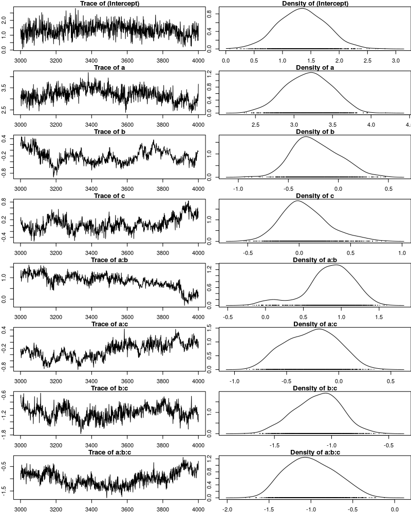
There are signals in these plots suggesting that our sample may not be good. In general, there is high autocorrelation, which means that samples tend to have similar values as the directly preceding samples. Also the traces are not stationary, which means that the sampling process dwells in one part of the parameter space and then visits other parts of the parameter space. This can be observed at around 3900 samples where the trace of c suddenly moves to more positive values not visited before and the trace of a:b moves to more negative values. Think about it this way: looking at these plots, is it likely that the density plots on the right would change if we would continue taking samples? Yes, it is because there may be more sudden moves to other parts of the parameter space like that at around 3900. Or the sampling process might dwell in the position reached at 4000 for a longer time leading to a shift in the distributions. For example the density plot of a:b has a long tail coming from the last ~100 samples and this tail might have gotten fatter if we hadn’t ended the sampling process at 4000 (later we will see that this is exactly what happens). As long as these density plots keep changing, the sampling process has not converged and we don’t have a stable posterior.
Ideally, we would like to have something like the following:
set.seed(1)
par(mfrow=c(1,2), mar=c(2,2,1,0))
x <- rnorm(1000)
plot(3001:4000, x, t="l", main="Trace of x")
plot(density(x), main="Density of x")
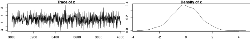
In this trace plot of random data, there is no autocorrelation of consecutive samples and the distribution of samples is stationary. It is very likely that taking more samples wouldn’t shift the distribution substantially. Hence, if we see a plot like this, we would be more confident that our posterior is a good approximation of the true posterior.
How can we reduce autocorrelation? One simple way is thinning. Autocorrelation decays over time, meaning that the correlation of samples tends to be lower the further apart two samples are. Therefore we can lower the autocorrelation by keeping only every n-th sample and discarding the samples in between. The thinning factor is then n. Of course, thinning also requires that we run the sampling process longer to obtain a large-enough set of usable samples.
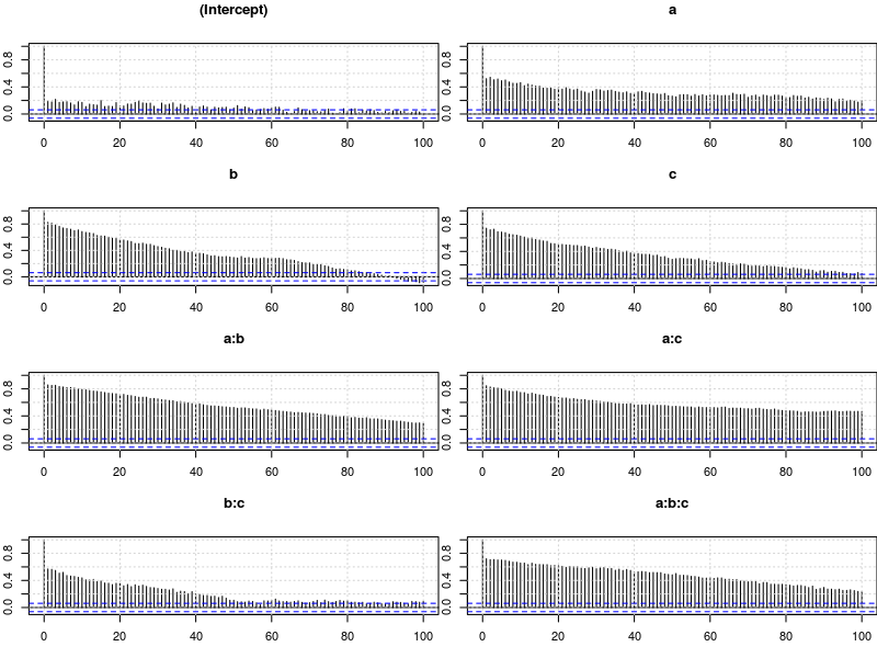
Let’s have a look at the autocorrelation of samples obtained with the model above. The plots below show for each parameter the autocorrelation as a function of the distance between samples. If the distance is 0, the autocorrelation is one because the correlation of a variable with itself is one. However, as the distance between samples increases the autocorrelation diminishes. We also see that the parameter for the intercept has much lower autocorrelation than the other parameters.
plot.acfs <- function(x) {
  n <- dim(x)[2]
  par(mfrow=c(ceiling(n/2),2), mar=c(3,2,3,0))
  for (i in 1:n) {
    acf(x[,i], lag.max=100, main=colnames(x)[i])
    grid()
  }
}
plot.acfs(m3$Sol)
Now let’s see what happens when we increase the thinning factor from 1 to 20 (thin=20). To compensate for the samples that we lose by doing so, we also increase nitt from 4000 to 23000 (3000 burn-in samples plus 20000 samples of which we keep every twentieth).
set.seed(1)
m4 <- MCMCglmm(pronoun ~ (a + b + c)^3,
                       ~ us(1 + (a + b + c)^3):subject +
                         us(1 + (a + b    )^2):item,
               data   = d,
               family = "categorical",
               prior  = prior.m3,
               thin   = 20,
               burnin = 3000,
               nitt   = 23000)
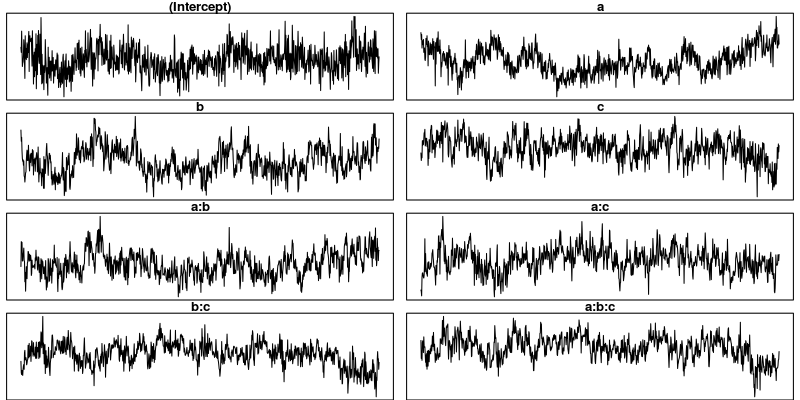
Examining the plots of the traces, we see that the autocorrelation is indeed much lower and the traces also look much more stationary than before. Inferences, based on this sample are therefore more trustworthy than inferences based on our earlier sample. However, the plots of the autocorrelation shows that there is still a great deal of it.
trace.plots <- function(x) {
  n <- dim(x)[2]
  par(mfrow=c(ceiling(n/2),2), mar=c(0,0.5,1,0.5))
  for (i in 1:n) {
    plot(as.numeric(x[,i]), t="l", main=colnames(x)[i], xaxt="n", yaxt="n")
  }
}
trace.plots(m4$Sol)
plot.acfs(m4$Sol)
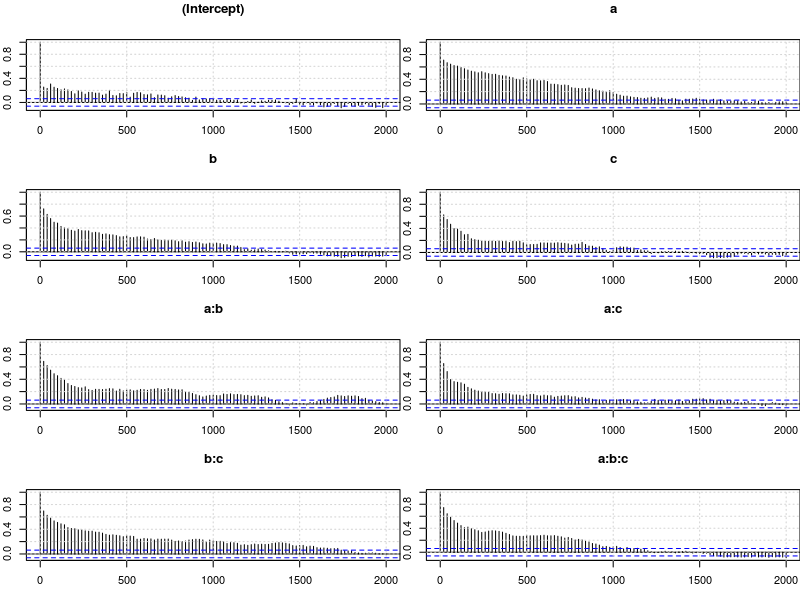
At this point, we have to ask: What is the cause of the high autocorrelation? The most likely explanation is that the data is not constraining enough to inform us about the relatively large number of parameters in the model. If that’s the case, one thing we can do is to reduce the number of parameters. Below, we fit a model that has only random intercepts and the random slopes for the effects of interest (the three-way interaction) but no random slopes for the main effects and their two-way interactions.
prior.m5 <- list(
  R=list(V=1, n=1, fix=1),
  G=list(G1=list(V        = diag(2),
                 n        = 2,
                 alpha.mu = rep(0, 2),
                 alpha.V  = diag(2)*25^2),
         G2=list(V        = diag(2),
                 n        = 2,
                 alpha.mu = rep(0, 2),
                 alpha.V  = diag(2)*25^2)))

m5 <- MCMCglmm(pronoun ~ (a + b + c)^3,
                       ~ us(1 + a : b : c):subject +
                         us(1 + a : b    ):item,
               data   = d,
               family = "categorical",
               prior  = prior.m5,
               thin   = 20,
               burnin = 3000,
               nitt   = 23000)
trace.plots(m5$Sol)
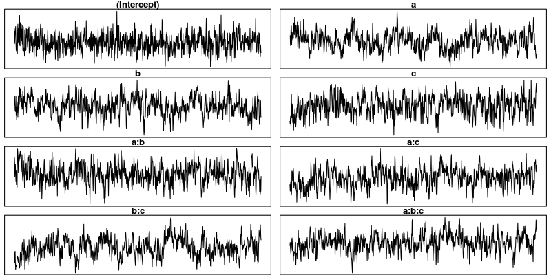
plot.acfs(m5$Sol)
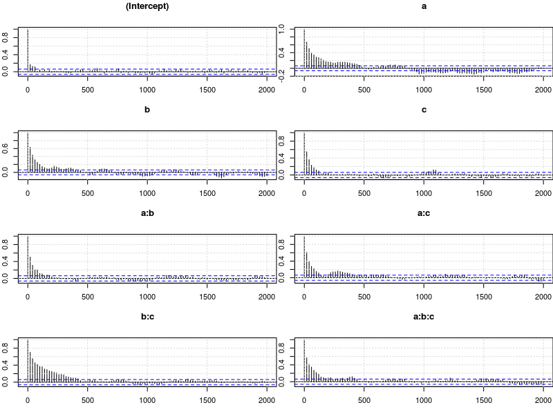
This looks much better than what we had before but the situation is still somewhat unsatisfying because so far we have no objective test for determining whether the obtained samples are good enough. The Gelman-Rubin criterion is such an objective test.
Gelman-Rubin criterion
The idea is to run multiple chains and to check whether they converged to the same posterior distribution. Since the sampling process is stochastic this is not expected to happen by chance but only when the data was constraining enough to actually tell us something about likely parameter values.
Below we use the package parallel to run four chains concurrently. This is faster than running one after the other because modern CPUs have several cores that can carry out computations in parallel. The chains are collected in the list m6.
library(parallel)

set.seed(1)
m6 <- mclapply(1:4, function(i) {
  MCMCglmm(pronoun ~ (a + b + c)^3,
                   ~us(1 + a : b : c):subject +
                    us(1 + a : b)      :item,
           data   = d,
           family = "categorical",
           prior  = prior.m5,
           thin   = 20,
           burnin = 3000,
           nitt   = 23000)
}, mc.cores=4)

m6 <- lapply(m6, function(m) m$Sol)
m6 <- do.call(mcmc.list, m6)
The coda package provides a lot of functions that are useful for dealing with Markov chains and it also contains an implementation of the Gelman-Rubin criterion (along with a number of other criteria). For those who are interested, the documentation of gelman.diag contains a formal description of the criterion.
The test statistic is called the scale reduction factor. The closer this factor is to 1, the better the convergence of our chains. In practice, values below 1.1 can be acceptable and values below 1.02 are good. In the plots below, the scale reduction is shown for bins of increasing size (1 to 50, 1 to 60, etc.), thus showing how the scale reduction factor develops over time. 97.5% confidence intervals are indicated by the red dashed line. Note that the x-axis shows the original indices of the samples before thinning.
library(coda)

par(mfrow=c(4,2), mar=c(2,2,1,2))
gelman.plot(m6, auto.layout=F)
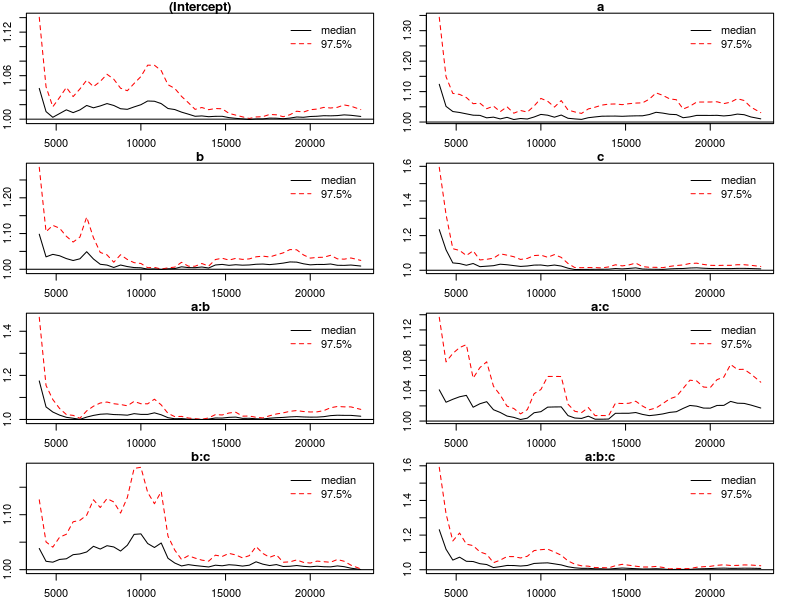
The plots suggest that the chains converged well enough after roughly half of the samples (after thinning), we say that the chains are mixing at that point. The function gelman.diag computes the scale reduction factors for each parameter and an overall (multivariate) scale reduction factor. All values suggest that our chains are good to be interpreted.
gelman.diag(m6)
Potential scale reduction factors:

            Point est. Upper C.I.
(Intercept)       1.00       1.01
a                 1.01       1.03
b                 1.01       1.02
c                 1.01       1.02
a:b               1.01       1.05
a:c               1.02       1.05
b:c               1.00       1.00
a:b:c             1.01       1.02

Multivariate psrf

1.04
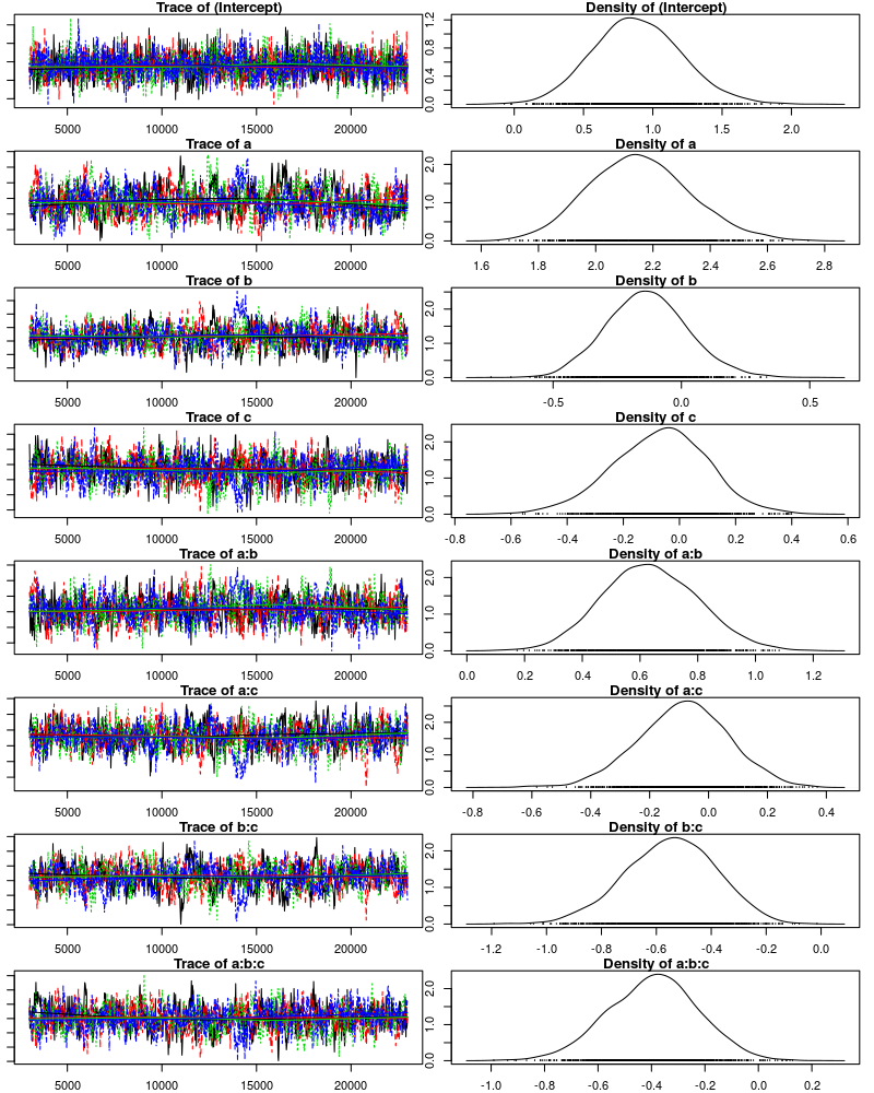
We can also visually confirm that the chains are mixing. Below each chain is plotted in a different color and we see that all chains visit the same parts of the parameter space.
par(mfrow=c(8,2), mar=c(2, 1, 1, 1))
plot(m6, ask=F, auto.layout=F)
Results
Having established that our sample is a good approximation of the posterior distribution, we can now move on and examine the results. We first look at the posterior means and the quantiles for each parameter.
summary(m6)
Iterations = 3001:22981
Thinning interval = 20
Number of chains = 4
Sample size per chain = 1000

1. Empirical mean and standard deviation for each variable,
   plus standard error of the mean:

                Mean     SD Naive SE Time-series SE
(Intercept)  0.88924 0.3213 0.005081       0.008347
a            2.15382 0.1762 0.002786       0.009356
b           -0.13308 0.1589 0.002513       0.007279
c           -0.07015 0.1693 0.002676       0.006484
a:b          0.63598 0.1649 0.002608       0.006734
a:c         -0.08589 0.1541 0.002436       0.006564
b:c         -0.54825 0.1651 0.002610       0.008497
a:b:c       -0.39332 0.1684 0.002663       0.006357

2. Quantiles for each variable:

               2.5%     25%      50%      75%    97.5%
(Intercept)  0.2844  0.6706  0.87936  1.09855  1.54454
a            1.8300  2.0299  2.14763  2.26796  2.51651
b           -0.4322 -0.2408 -0.13649 -0.03014  0.19503
c           -0.4219 -0.1855 -0.06182  0.04427  0.25302
a:b          0.3280  0.5246  0.63149  0.74883  0.96597
a:c         -0.3960 -0.1856 -0.08108  0.01903  0.20818
b:c         -0.8833 -0.6597 -0.54194 -0.43252 -0.24247
a:b:c       -0.7308 -0.5079 -0.38878 -0.28100 -0.07177
And here is a plot of the posterior means along with 95% credible intervals:
plot.estimates <- function(x) {
  if (class(x) != "summary.mcmc")
    x <- summary(x)
  n <- dim(x$statistics)[1]
  par(mar=c(2, 7, 4, 1))
  plot(x$statistics[,1], n:1,
       yaxt="n", ylab="",
       xlim=range(x$quantiles)*1.2,
       pch=19,
       main="Posterior means and 95% credible intervals")
  grid()
  axis(2, at=n:1, rownames(x$statistics), las=2)
  arrows(x$quantiles[,1], n:1, x$quantiles[,5], n:1, code=0)
  abline(v=0, lty=2)
}

plot.estimates(m6)
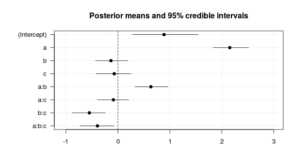
As we can see, the three-way interaction is significant. Some other effects are significant, too, but note that we should be careful in interpreting these effects because the model does not include the relevant random slopes and may therefore overestimate the reliability of these effects (see Barr et al., 2013, for details).
Summary
Our attempts to analyze the data with lme4 failed due to convergence errors. Even a radical simplification of the random effects structure did not help. In contrast to that the Bayesian mixed-effects model converged fine after a simplification of the model and a few adjustments to the sampling process. The price for this was that we had to take more control of the model fitting process than we have to when working with lme4 which tries to handle all that automatically. In sum, MCMCglmm is a powerful tool that can be used when lme4 has convergence problems or when models are desired that are outside the scope of what lme4 can do.
References
- Barr, D. J., Levy, R., Scheepers, C., & Tily, H. J. (2013). Random effects structure for confirmatory hypothesis testing: Keep it maximal. Journal of Memory and Language, 68(3), 255–278. http://dx.doi.org/10.1016/j.jml.2012.11.001
- Bates, D., Kliegl, R., Vasishth, S., & Baayen, H. (2015). Parsimonious mixed models. Manuscript published on arXiv. http://arxiv.org/abs/1506.04967
- Gelman, A., & Rubin, D. B. (1992). Inference from iterative simulation using multiple sequences. Statistical Science, 7(4), 457–472.
- Hadfield, J. (2010). MCMC methods for multi-response generalized linear mixed models: the MCMCglmm R package. Journal of Statistical Software, 33(1), 1–22. https://cran.r-project.org/web/packages/MCMCglmm/vignettes/Overview.pdf
- Hadfield, J. (2015). MCMCglmm Course Notes. https://cran.r-project.org/web/packages/MCMCglmm/vignettes/CourseNotes.pdf